Quick start

If it's your first time using EcologicalNetworksDynamics, exploring this example might be useful to you so that you understand how the package works. Try pasting the following code blocks in a Julia terminal.

The first step is to create the structure of the trophic interactions.

using EcologicalNetworksDynamics, Plots
fw = Foodweb([1 => 2, 2 => 3]) # 1 eats 2, and 2 eats 3.

blueprint for Foodweb with 2 trophic links:
  A:
  1 eats 2
  2 eats 3

Then, you can generate the parameter of the model (mostly species traits) with:

m = default_model(fw)

Model (alias for EcologicalNetworksDynamics.Framework.System{<inner parms>}) with 17 components:
  - Species: 3 (:s1, :s2, :s3)
  - Foodweb: 2 links
  - Body masses: [100.0, 10.0, 1.0]
  - Metabolic classes: [:invertebrate, :invertebrate, :producer]
  - GrowthRate: [·, ·, 1.0]
  - Carrying capacity: [·, ·, 1.0]
  - ProducersCompetition: 1.0
  - LogisticGrowth
  - Efficiency: 0.45 to 0.85.
  - MaximumConsumption: [8.0, 8.0, ·]
  - Hill exponent: 2.0
  - Consumers preferences: 1.0
  - Intra-specific interference: [·, ·, ·]
  - Half-saturation density: [0.5, 0.5, ·]
  - BioenergeticResponse
  - Metabolism: [0.09929551852928711, 0.1765751761097696, 0.0]
  - Mortality: [0.0, 0.0, 0.0]

For instance, we can access the species metabolic rates with:

m.metabolism

3-element EcologicalNetworksDynamics.MetabolismRates:
 0.09929551852928711
 0.1765751761097696
 0.0

We see that while consumers (species 1 and 2) have a positive metabolic rate, producer species (species 3) have a null metabolic rate.

Use properties to list all properties of the model:

properties(m)

63-element Vector{Any}:
 :A
 :K
 :M
 :S
 :body_masses
 :carnivorous_links
 :carrying_capacity
 :consumers_dense_index
 :consumers_indices
 :consumers_mask
 ⋮
 :tops_dense_index
 :tops_indices
 :tops_mask
 :tops_sparse_index
 :trophic_levels
 :trophic_links
 :w
 :x
 :y

At this step we are ready to run simulations, we just need to provide initial conditions for species biomasses.

B0 = [0.1, 0.1, 0.1] # The 3 species start with a biomass of 0.1.
t = 100 # The simulation will run for 100 time units.
out = simulate(m, B0, t)

retcode: Success
Interpolation: 3rd order Hermite
t: 36-element Vector{Float64}:
   0.0
   0.11699364210598083
   0.48617832763452
   1.0368468338830605
   1.7139555674399034
   2.5513962727226556
   3.5330334816834155
   4.505265250256067
   5.836074084549767
   6.967915760126519
   ⋮
  67.11317082453247
  71.58230021827859
  76.07250167329737
  80.79722378308718
  85.6102128199706
  90.25459748182507
  94.79677297455524
  99.46550578816947
 100.0
u: 36-element Vector{Vector{Float64}}:
 [0.1, 0.1, 0.1]
 [0.09919287669046291, 0.09822884333138167, 0.10943428041997874]
 [0.09662179888206167, 0.09376940946687998, 0.14338556886802853]
 [0.09279833849415957, 0.09092616703154523, 0.20497788294832414]
 [0.08831859508269191, 0.09550058444526696, 0.291897475007018]
 [0.08358086784237422, 0.11717295207958495, 0.39129687468493096]
 [0.08033574328747636, 0.1698979316215357, 0.4473504571406456]
 [0.08170432197861595, 0.24640046743456728, 0.41360402397358736]
 [0.09414437138395253, 0.33526354499904654, 0.30392418756145695]
 [0.11304463444268815, 0.35620385298488444, 0.24559294542421828]
 ⋮
 [0.6301062715133536, 0.1909967383072635, 0.4105099776998821]
 [0.6351156117692149, 0.19056203525059076, 0.41177313089869216]
 [0.6388745813719467, 0.1902436697575823, 0.4128818738635837]
 [0.641835999157327, 0.18998735120427251, 0.41379621984792614]
 [0.6440402600848345, 0.1897987300754866, 0.41457765902356014]
 [0.6456251919424584, 0.18958550024079587, 0.4152409717101538]
 [0.6468489789602436, 0.18936158693413355, 0.41566297918003764]
 [0.6478264417019027, 0.18918126317278258, 0.4159068868770515]
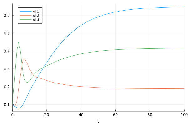
 [0.6478951500465029, 0.18921365317121666, 0.41592749130883]

Lastly, we can plot the biomass trajectories using the plot functions of Plots.

plot(out)